Causality Analysis
Using the MBTI personalities to assess Barbenheimer
 Don’t worry, we’ve reached the final part of our analysis: soon you can go back to beach, not surfing, just BEACH…
Building up on our previous plots and analyses on genre and character types, we now want to acknowledge the reliability of our data comparisons. This is why we are performing a causality analysis.
Research Question
In this section we'll discuss the following question:
- What are the influences of various movie parameters on its succes?
How do we define success?
We have identified two main indicators of the success of a movie. First, the average rating of the movie provided by IMDb, that should represent the popular opinion about this movie.
However, unless they have a strong opinion about a movie, most people don't take the time to express their views and therefore, the ratings might not be the perfect representation.
The second indicator is the Box Office Revenue, as success could be defined by how popular the movie is. One could also argue that some genres are more popular than others and would gross more,
and therefore doesn't give an idea of the quality of the movie. We decided to measure if ratings and grossing were correlated in some ways. For that, we
conducted a linear regression on our data and found the following results:
Analysis on diversity
We decided to group the data manually into broader ethnic groups for more meaningful conclusions. The following histogram portrays the ethnicities of all actors in the movies dataset. First and foremost, we can see that caucasians make up the vast majority of actors (e.g., Margot Robbie as Barbie, Ryan Gosling as Ken and Cillian Murphy as Robert J. Oppenheimer), followed by african, and other ethnicities, who are in the minority.
We decided to see if diversity, measured by the number of different ethnicities in a movie, had an impact on the success of that movie. The first violin plot tests the comparison of the number of different ethnicities in a movie and the revenue generated from the movie. What is observed is that as the number of ethnicities increases, the movie tends towards a higher revenue. We can also notice that the data is unevenly distributed, as most movies have a maximum of three different ethnic groups. We computed a linear regression and found a slope of \(\beta_1 = 3.33 \cdot 10^7\) and an intercept of \(\beta_0 = 2.37 \cdot 10^7\), with a p-value of \(p = 3.36 \cdot 10^{-214}\) and \(R^2 = 0.033\). Once again, the low p-value combined with a low R-squared value indicate a weak correlation between both parameters.
The second plot compares the movie rating to the number of different ethnicities:
Again, by disregarding the outliers stemming from movies with five or six different ethnicities, we observe that the ratings maintain similar ratings, thus reinforcing that the number of diversity does not impact movie ratings. The linear regression yields \(\beta_1 = -0.12\) and an intercept of \(\beta_0 = 6.62\), with a p-value of \(p = 6.26 \cdot 10^{-66}\) and \(R^2 = 0.010\), giving an even weaker correlation since R-squared is very low and the slope is almost null.
Let's compare ethnic groups!
We decided to measure the effect of the ethnicities of the cast in a movie. We previously looked at the diversity, let's now find out about ethnicity. Since the distribution of ethnicities is very skewed, a Kruskal-Wallis test was conducted to fortify the analysis for both Box Office Revenue and Ratings, and the p-values found are respectively \(p = 7.61 \cdot 10^{-11}\) for Revenues, and \(p = 9.22 \cdot 10^{-42}\) for Ratings. This allows to test if we can reject the null hypothesis: all ethnic groups have the same median revenue/rating. Since the p-values are very low, we conclude that the ethnicities do not all have the same revenue, and this can be observed through the interactive box plot.
For Movie rating versus different ethnicities, we also came up with the conclusion that different ethnicities do not have the same ratings.
We can observe that the repartition of ethnicities is skewed, as there are much more caucasians as opposed to other ethnicities. The Kruskal-Wallis test is non-sensitive to the distribution of the data, however it is a non-parametric test and only give us the information that at least one category doesn’t have the same median, but we do not know how many and which ones.What about release years?
Remember Barbenheimer? Fun fact: they were both released on the same day, the 21st of July 2023 (in the USA)! Was it a tough decision for you which one to watch first or did you have a preference from the start?

To continue our investigation on the factors of success, we can look at the influence of the realease year over Box Office Revenue and Ratings. The following scatter plot compares the Revenue of a movie to the release year. We computed a linear regression and got the following results: \(\beta_1 = 1.06 \cdot 10^6\) and an intercept of \(\beta_0 = -2.06 \cdot 10^9\), with a p-value of \(p = 2.25 \cdot 10^{-65}\) and \(R^2 = 0.034\). The conclusion remains the same, there is a weak correlation between Revenues and Release Year. This might be due to many different factors (inflation, popularity of cinema).
Finally, we can compare the ratings of movies to their release year. We computed a linear regression and got the following results: \(\beta_1 = -0.0009\) and an intercept of \(\beta_0 = 7.95\), with a p-value of \(p = 4.99 \cdot 10^{-7}\) and \(R^2 = 4.2 \cdot 10^{-4}\). The value of the slope indicates that there is almost no correlation between Ratings and Release Year. This can be due to the fact that ratings can be submitted anytime so the effect of time isn't as strong as it is for revenues.
What is observable is that the grossing increases throughout the years and the ratings have remained even.Do characters archetype affect the popularity?

What is the biggest difference between Barbie and Oppenheimer? That's right, personality. In our endless search for factors of success, we will now use the results from the MBTI analysis to determine if having extroverted characters boost the Ratings and Revenues.
Let's first look at the plot of Ratings against the proportion of extroverted characters in a movie. Here we have both a barplot with 95% confidence intervals and a scatter plot of all the data points. Looking at the bar plot we may think that there is lower rating as extroversion proportion increases but running a Chi-squared test returns a p-value of 0.2328 showing that the differences in average ratings are not statistically significant.

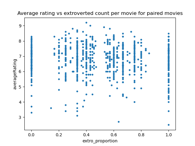
At first sight, it seems that movies with extroverted characters might have slightly worse ratings than movies with introverted characters. The correlation, if it exists, would be weak. Let's now try pair matching to eliminate covariates and draw meaningful conclusions. We matched movies along many parameters, such as genre, release year, number of characters, number of votes for rating. Since the proportion of extroverted characters is not a binary variable, we also matched movies with the same proportion of one type so that we require "in a pair, movie 1 has as many extroverted characters as movie 2 has extroverted characters". We used a mix of methods, exact matching when possible (eg. number of characters) and also propensity score matching (number of votes, release year).
After performing the linear regression we obtain a slope coefficient of -0.2232 which isn't a very strong correlation and the p-value for it is 0.042 which makes the result statistically significant. However we do notice the R-squared value of 0.005 is extremely low which means that extroverted proportion explains almost none of the variance in average rating. On the scatter plot below, which shows only the paired movies, we see that there is still no trend that appears, meaning there could possibly be even more covariates that we did not take into account. We also see in the bar plot that there is still no trend appearing in the data.
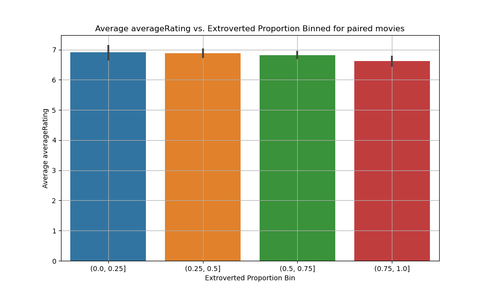
Once again if we look at the bar plot and run a Chi-squared test we see that the differences in average ratings is not statistically significant so we cannot reject the null hypothesis which is that average rating is the same for all bins.
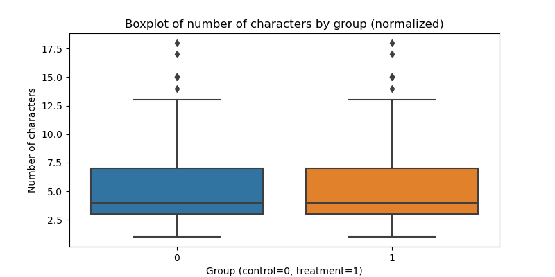
Now of course, when pairing datapoints together, we have to check the balance between our treatment and control groups. This is validated by the plots below.
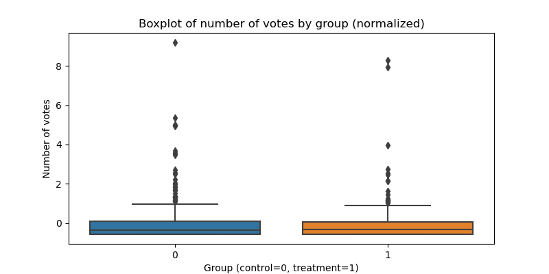
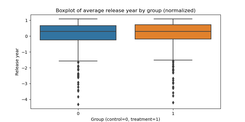
So at the end of it all we could get a causality diagram that looks like this, as you can see there are very many links that need to be investigated and even though our analysis barely scratched the surface we already can identify many variables that could affect movie success.
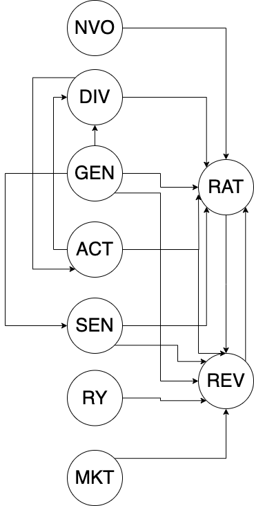
With NVO - Number of votes, DIV - Diversity, GEN - Genre, ACT - Actors, SEN - Sentiment, RY - Release year, MKT - Marketing, RAT - Average Rating, REV - Movie Revenue.